A Calculator (7): Writing Microcode for a CPU You Just Invented

In the previous post, we designed the CPU. We settled on the instruction set, wrote the assembler, verified each opcode, and ended up with a clean, working processor running in silicon (or rather, in an Altera Cyclone II EP2C5T144C8 FPGA, which is close enough). What we did not have yet was a meaningful software – the calculator microcode – to run it on.

Building on Our Earlier Work

This is the part of the project where all those C++ prototype experiments described in posts 2 and 3 paid off.

When I started writing addsub.asm (the very first function I ported), I was not staring at a blank page wondering how BCD addition works. I had a reference implementation in C++ (addsub.cpp in the Proto project) that I had already verified against thousands of test vectors. The algorithm was known, the edge cases were found and characterized. The guard digit and sticky bit behavior had been worked out. All I had to do was translate it into assembly – which is still genuinely hard, but it is a very different kind of hard from discovering the algorithm while also writing it.

I want to emphasize such two-stage approach because it may be tempting to skip. Writing prototype code in C++ and then hand-translating it to assembly feels redundant and a lot of work. However, it does not feel redundant by the time you are debugging the third subtle rounding edge case in a 16-nibble BCD subtraction. Having a golden reference you can run against is not optional: it is the only thing standing between you and weeks of confusion or even giving up.

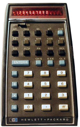
The history of HP’s own calculator software should be enough to convince anyone. The first production run of the HP-35 shipped in 1972 with a bug where typing 2.02 ln ex produced 2 instead of 2.02. The numerical algorithms in that machine had no automated test vectors to catch the edge case — HP engineers had been validating results by hand against printed tables, and this particular value slipped through. When the bug was discovered, one of the founders reportedly snapped his pencil when someone in the meeting suggested simply not telling customers. HP offered free replacements to all affected owners. Only about 25% returned their calculators — but the lesson about rigorous numerical testing had been learned the hard way.

The calctest utility (covered in Post 4) made this easier. Running calctest against a new function tells you immediatly whether the microcode matches the prototype. When you make a mistake in the assembly, you know exactly which case failed, rather than hunting through a pile of symptoms.

The Three Faces of the Calculator Microcode

In the current edition, about two dozens of assembly files make up the microcode. They can be grouped into three distinct concerns, separate not just organizationally but conceptually: each one has different inputs, different outputs, and a different style of complexity. (A fourth module, the scripting layer, is covered in its own section below.)

1. Number Input

input.asm handles everything that happens between the user pressing a key and a well-formed number appearing in the X register. The list of cases it must get right is longer than you might expect: leading zeros, the decimal point (only one allowed!), the sign (can appear before the mantissa or the exponent), the exponent separator, switching from mantissa entry to exponent entry mid-number, rejecting additional digits when the display is full, handling CHS (change sign) differently depending on whether you are entering the mantissa or the exponent. One level up, it needs to handle stack lift semantics: whether pressing a digit after ENTER pushes the current X or overwrites it, along with the rest of user stack manipulation.

The input module is also responsible for deciding which mode a digit press is in. Pressing 5 can mean: enter the digit 5 into the number being typed; set the display precision to 5 digits if the user is in DISP mode (the interactive format and precision selector); or select memory register 5 if the user pressed STO or RCL. A single entry point handles all three cases by reading a state variable at the start. You have to get all the state transitions right.

The Pathfinding/Input C++ prototype was essential here. The input state machine has enough edge cases that debugging it directly in assembly would have been painful. The C++ version uses variable names that map directly to the assembly registers they will become Si_r3 for the screen index (eventually register R3), Mi_r5 for the mantissa index (R5), Di_r2 for the decimal point position (R2). This deliberate naming convention made the eventual assembly port almost mechanical: every variable in C++ had a pre-assigned register waiting for it. The heuristic was fully worked out and tested in C++ before a single line of assembly was written.

2. Display Output

Display output, with its various modes, is equally complex. display.asm is the single largest file in the entire project (larger than the addition/subtraction, larger than the logarithm, larger than anything else).

The calculator supports three decimal display modes (Fixed, Scientific, Engineering) plus Raw (all 16 mantissa digits, useful for debugging or when you want to see all the resulting digits). Each mode has its own formatting rules. Engineering mode, for example, keeps the exponent as a multiple of 3 and adjusts the mantissa position accordingly: 0.1234 displays as 123.4 E-03 rather than 1.234 E-01, because engineers think in millis and micros and want to read directly in SI units. (If that seems simple, wait until you have to implement it.)

Rounding is also done here and not on user registers. This is deliberate: you want the internal registers to retain full 16-digit precision, but the display can show less than that. The rounding step has to handle the carry-propagation case where rounding up the last displayed digit causes it to become 10, which ripples leftward and may even change the magnitude (exponent) of the number, which in turn may hit the upper limit of what we can display. At the extreme, this rounding can make the result cause the overflow in which case we display the largest value possible. This rounding-induced “overflow” is different from a “true” overflow that shows as an error.

I wrote this module last, after input and the basic calculations were working, precisely because I knew it would be the hardest. This is the only module for which I did not have C++ reference. By that time, I became very good at writing assembly code, so I just winged it.

3. Calculation in Assembly

This is the core of the calculator. The assembly code maps almost directly onto the C++ prototype files from earlier in the project. For each basic function there is a corresponding assembly file:

• addsub.asm — addition and subtraction, with guard digit and sticky bit
• mul.asm — the nibble-by-nibble multiplication algorithm (table driven)
• div.asm — shift-and-subtract long division
• sqrt.asm — Square root using Newton-Raphson iteration
• log.asm / exp.asm — HP-style pseudo-division/multiplication CORDIC
• tan.asm / atan.asm / atan2.asm — decimal CORDIC tangent
• sin.asm / cos.asm — derived from CORDIC tangent

The CORDIC algorithm has an interesting origin. Jack Volder conceived it in 1956 (we covered the algorithm itself in Post 3; what follows is the story behind it) while working at Convair’s aero electronics department, where the task was replacing an analog resolver in the B-58 Hustler supersonic bomber’s navigation computer with a faster digital system. He published the results in the IRE Transactions on Electronic Computers in 1959. For years it remained a niche technique used in military navigation systems. Then in 1971, John Stephen Walther at Hewlett-Packard generalized the algorithm to handle hyperbolic functions, logarithms, and exponentials using the same shift-and-add structure. That generalization, published in the spring of 1971, fed directly into the HP-35 the following year (the world’s first scientific pocket calculator).

Each of my assembly files began as a direct port of the equivalent C++ functions in the Proto project. The process was: read the C++ carefully, follow the data flow (which registers hold what, and in what format), and then write the assembly strictly following the reference code flow, line by line, operation by operation. I was even keeping the same comments, verbatim, so the sources would roughly look similar. That all helped debugging occasional problems – which I really did not have many due to the rigor.

The test vectors from Proto, fed through calctest, confirmed when the port was faithful. For difficult cases, I used Qt app to debug a test vector.

While the C++ prototype provided raw functionality heuristic, it still lacked main calculator wrapper and structure.

This is an example of part of that structure. Here is the actual entry point from addsub.asm:

pre_calc_2 clears the input flag, saves LASTX, copies Y and X into scratch registers S0 and S1, and pops the user stack. addition runs the operation. post_calc_finalize re-enables stack lift, checks for errors, and copies the result register back to X.

The guiding principle was that each operation should expect one or both parameters in the scratch registers S0 and S1, and it should store its result to another scratch register called R (as in ‘result’). The upper level wrapper manages user-visible registers X, Y, Z, T and LastX.

This layered structure makes individual functions easier to test and swap out independently, but the most important benefit is that you can chain them since they have consistent interface with the rest of the system. This frictionless chaining allowed for a simple scripting language.

The Scripting Layer

Once the basic arithmetic and transcendental functions are working in assembly, a large number of the remaining calculator keys are simply combinations of those functions. y^x is e^(x * ln(y)). Reciprocal is 1 / x. Factorial iteratively multiplies by a countdown counter. Degrees-to-radians is a multiplication by a constant.

Writing each of these in assembly would be tedious and wasteful of ROM. Instead, the calculator has a small scripting interpreter. Scripts are stored in the data address space (in their own 2048-nibble ROM region), and the scripting engine processes 4-bit tokens that represent operations: Plus, Minus, Multiply, Divide, Loge, Expe, Copy, If_Goto, and so on.

The scripting engine is stack based (there are Push and Pop tokens), but it can also operate on registers directly (for example, it can load a constant into any user or scratch register). It assumes and follows the established contract that each operation expects its arguments in S0/S1 scratch registers and it leaves its result in R scratch register – which is also automatically copied to S0/S1 for the chained operation.

This idea is not new. Sinclair used exactly the same approach in the ZX81 and ZX Spectrum micros to implement floating-point math. Z80 has no floating-point instructions, so Sinclair’s ROM contains a small interpreter that processes a table of single-byte tokens (each one dispatching to a short assembly routine for operations like addition, multiplication, sine, or logarithm). Complex calculator functions in the BASIC interpreter are then expressed as compact sequences of those tokens rather than as repeated inline assembly. Dr. Steve Vickers, who wrote the Spectrum ROM at age 27 entirely in assembly, used this technique to squeeze a complete scientific calculator’s worth of math into a few kilobytes.

What makes the Spectrum’s version particulary elegant is its invocation mechanism: a Z80 program calls the floating-point calculator simply by executing RST 28H, then placing a stream of token bytes in the code immediately following that call. The interpreter reads those bytes, processes each operation, and returns with the result on the floating-point stack. The entire BASIC interpreter’s expression evaluator and all scientific functions are expressed in this way. Vickers was, in effect, implementing a small virtual machine inside the ROM. That Forth-like, stack-based design apparently captured his thinking so thoroughly that his next project after leaving Sinclair was the Jupiter Ace (a home computer that shipped with Forth as its primary language rather than BASIC), a language whose stack-based token dispatch is the direct philosophical descendant of the Spectrum’s calculator VM. It is still studied today by anyone who reverse-engineers the Spectrum ROM.

Our scripting is also very compact. The result is that a function like sc_ypowx (y raised to the power x) looks like this:

Six lines. That is the complete implementation of y^x, once Loge and Expe exist in assembly. The scripting language sits on top of the assembly layer like a macro system, and a surprisingly large fraction of the calculator’s 35-key layout is implemented at that level.

The exchange function (sc_exchg, swap X and Y) takes four lines; the RPN stack roll is six lines. Factorial is about twenty-five, including the loop and argument validation. Degrees-to-radians is a multiply by the constant π/180, and so on.

We discussed this in The Numerical Methods post earlier: you can get “36 operations for the price of 8”. The scripting layer enables that. With Loge, Expe, Sqrt, and the four basic operations, you can express most of a scientific calculator operations. The interpreter and the script it runs complete all the higher functions that would otherwise each need their own assembly implementation.

The scripting compiler is implemented as a Python script (cscript.py), sister tool to the assembler. It reads .scp files, resolves labels, and outputs packed 4-bit tokens in the same $readmemh-compatible format that the assembler uses. When I initially thought of the script compiler the obvious choice was to simply copy already existing assembler (casm.py) and then strip all assembler mnemonics and add scripting tokens. A few minor adjustments later, and the scripting compiler had enough capability to handle scripting language and produce scripting tokens.

How the Interpreter Works

The interpreter code takes a few dozen lines of assembly in scripting.asm. The core loop is:

aload reads one word (a nibble) from the data address pointer and advances it. tblcall uses R0 as an index into a jump table and calls the corresponding routine. That is the gist of the engine. The complexity lives in the dispatch tables and the handlers they point to, not in the loop itself. Several scripting tokens are also re-entrant, so a complex script can recursively call other scripted functions.

A scripting token is a 4-bit value, giving 16 possible opcodes per group. The token set is split into three groups to pack more operations into that narrow space. Group 0 are single-nibble instructions that take no additional arguments: the arithmetic operations, the basic flow control entry points, and two escape codes. Token 0xE is the escape into Group 1: one additional argument followed by a register index, flag index, or a trig function selector. Token 0xF is the escape into Group 2: two additional arguments followed by a destination and a source register. User registers are one of X, Y, Z, T, LX, R, S0–S4, STAT_N/M/S/SUMX/SUMX2.

The complete token tables (all three groups, test operations, user register names, and constant indices) are in the Scripting Language Reference in the repository’s docs/ folder.

The Test token deserves a mention. It tests a register against one of six conditions (zero, negative, equal to S0, numeric error, invalid, or greater-than-or-equal to S0) and stores the boolean result in FLAG_TEST. This single token makes conditional branching possible in scripts without exposing the CPU’s flag register directly.

To make this concrete, here is factorial, which is one of the more complex scripts and uses most of the language’s features:

There is a loop written in a language with no loop instruction. The Jump token provides unconditional redirection; If_Goto and If_Not_Goto provide conditional exits. The data stack (via Push and Pop) holds the accumulator across iterations. It reads clearly, compiles to a tight sequence of 4-bit tokens, and runs on the same interpreter that handles everything else just as elegantly.

The scripting layer ended up absorbing more and more functions over time. Operations that sometimes started in full assembly (statistical accumulators, HMS conversion, polar/rectangular conversion) migrated to scripts as the language grew more capable. In the end, most calculator’s functions run entirely in script, with assembly handling only the numerical primitives underneath.

My experience was that you don’t need too many control primitives for a scripting language for it to quickly become very usable. At the beginning, I had only a few and was able to implement a number of functions. Later, I started adding some more exotic ones, more for the kicks or because it was a very simple tweak on the already existing support.

However, it is always a good choice to be conservative, pragmatic and leave plenty of room for eventual expansion. Think wider, but implement minimally.

Debugging Microcode: The Qt Simulator

Writing microcode for a custom CPU has one particular hazard: when something goes wrong, you cannot simply add a print statement. The CPU does not know what print means.

To make this manageable, one of the very first thing I built was a Qt desktop application that runs the entire Verilog design through Verilator (the cycle-accurate C++ simulator we covered in an earlier post) and wraps it in a proper debugging environment. The calculator runs on your desktop with a full graphical keypad and an LCD display that accurately renders the HD44780U character set.

On the right side of the window sits the debug console. It accepts commands typed at a prompt, and even the familiar function keys work as expected: F11 single-steps one instruction, F10 steps over a subroutine call, F5 continues to the next breakpoint. These shortcut keys are read from a configuration file.

The debugger understands the microcode at source level. When you load a microcode listing file (generated by the assembler alongside the binary), the l command shows the original source lines:

Breakpoints accept either hex addresses or symbol names directly. For example, bp key_plus sets a breakpoint at the entry to the addition handler, bp division catches the divide routine. When a breakpoint hits, the console prints the address and the label name, so you always know where you are in the source, not just in the binary.

The r command dumps all CPU registers and flags. The d command dumps a region of RAM in nibble format, which is essential for inspecting calculator register contents mid-calculation. dr displays all user-facing registers (X, Y, Z, T, LastX and the scratch registers) formatted as BCD numbers, so you can see at a glance what values are in flight. ds shows the statistical accumulators. du shows the STO memory registers 0–9, and so on – press h for help.

There is also sr (set register) to inject a value directly into a calculator register from the console, and df to display the full 16-bit flag register. Together these let you set up a specific state, run to a point in the calculation, and inspect exactly what happened.

The testing framework integrates directly into the same console. tf tests.txt loads test vectors from the Proto C++ project, and te runs them against the live simulation. The same vectors that checked the C++ prototype now check the microcode on the actual simulated hardware.

The complete debugger command set, keyboard shortcuts, build instructions, and test framework details are in the Qt Simulator and Debugger Reference in the repository’s docs/ folder.

I cannot overstate how much time this saved. Microcode bugs tend to be subtle: a flag not cleared at the right moment, a register indexed one nibble off, a branch condition backwards. Without source-level debugging, tracking these down would be a very slow process. With it, most bugs reduced to setting a breakpoint near the suspect code, single-step through it, watching the registers and finding the line where something unexpected happens.

The same Qt application compiles to WebAssembly and runs in a browser, which is how the live demo on baltazarstudios.com works, and anyone can play with that online.

Microcode in Context

The microcode is not a static artifact. Between the initial 2021 implementation and my 2025 revision, the calculation algorithms were rewritten based on the improved Proto C++ reference: tighter guard digit handling, better rounding, the CALLI and other optimizations. Some functions were added (atan2, the statistical accumulators), some were restructured. The scripting layer absorbed more and more functions that had been in assembly.

The following set of graphs provide some insight into the microcode use of the CPU instructions.

The next post covers the physical hardware: boards, keypad, display, and the long journey from a breadboard to a self-contained battery-powered device. After that, the precision improvements of the 2025 revision. But if there is one thing I want the reader to take away from this post, it is this: writing microcode for a calculator is not just writing software. It is writing software in a language you invented, for a machine you built, to implement mathematics you verified from first principles. At every level, it is yours.

That is either terrifying or exciting, depending on your disposition. For me, it was definitely exciting. 🙂

---

All microcode source is in the ucode/ folder of the FPGA-Calculator repository. The calctest utility and test vectors are in calctest/.

---