This is the second article in a series on making our calculator. This article is about prototyping and the verification of fundamental algorithms.
We need to investigate and pick algorithms we will use and verify them against a known good, “golden” model. We need to code that. That platform also needs to be easy to use and debug. It should be quick to prototype various models so we can research different ideas before committing to them.
Usually, for such tasks, Python as a language of choice comes to mind, but for this project, I have selected C++ and MS Visual Studio’s basic console C++ project to construct such a framework. In my opinion, Visual Studio (Community Edition) is the best freely available debugging framework. When I was doing it, I also checked in the equivalent Makefile, so most projects can be compiled under Linux. Using both, I have also found certain discrepancies between the two compilers.
This step aims to verify the basic operations of addition, subtraction, multiplication, and division and the parsing of the input buffer. We want to investigate various ideas on how to do that effectively on BCD values, with mantissa and exponent processed separately. The code should be flexible and not tied to a particular mantissa width so that we can change it and see the impacts of such changes on the overall precision.
This code – a functional-level simulator – does not have to be too elaborate or fast. Quite the opposite: the goal is to start mimicking some low-level implementation that could be done in hardware so that the eventual translation, or conversion, may become more straightforward. Still, nothing is set in stone yet – as the verification progresses, it should become more apparent which parts would belong to what implementation level: whether an operation should be implemented in hardware or at the higher software level.
As I started work on this, gradually, some certainties about the internal architecture started to be apparent. Then, as you move in those directions, many related trade-offs seem to fall in place to form an architecturally consistent model. Some trade-offs are easier to make than others since they may be more obvious and likely to represent sound engineering reasoning. The harder ones require giving up some benefits to satisfy other variables (for example, selecting the mantissa or exponent widths).
Somewhere in that spectrum is a decision to use BCD as the internal number specification.
Why BCD?
While the binary floating-point (or IEEE 754 standard) is overwhelmingly used in general and scientific computation, fixed point BCD calculations are still very relevant in banking, finance, and commercial calculations due to their precision, accuracy, and immunity from implicit conversion errors. In many ways, doing arithmetic with BCD digits resembles calculating values as taught in school, on paper, digit by digit – there are no conversions to other number systems. Also, at any point in the process, digits are readily visible to a debugger, which makes the algorithms easier to debug.
Hence, mantissa will be stored in BCD format.
Exponents
Exponents, however, will be stored as 8-bit binary (integer) numbers. That format simplifies the operations that must be done with them – exponents are never addressed as individual digits. They are always used as integer numbers, so keeping them in a multi-digit BCD format would make their handling unnecessarily more complicated. Moreover, we will add a bias value of 128 to it. That will “move” their range to positive integers and simplify their comparisons.
Most calculators use a two-digit exponent, from -99 to +99, so we will also limit ours to that range. As they get internally converted to 8 binary bits, they will “lose” values in the ranges [0-28] and [228-255], and that is okay. (Maybe we could allow intermediate results to extend into those ranges.) Since exponents are always whole numbers (integers), we do not lose any precision when we convert them from a format of the two-digit input buffer to integers and back when we need to display their values. The process of such a 2-digit conversion is quite simple either way.
Note: The section above is now incorrect. I ended up storing exponents as pairs of BCD digits due to the characteristics of the CPU that I created for it. This is another proof of how things change during development!
Input parsing
This is the first practical operation that we need to code and verify. Inputting numbers is actually quite a complex operation. We need to handle digit insertion, deletion, switching the mode to exponent and back (as the user deletes digits of the exponent!), and also handling various edge cases. For example, the user could type a number too large to handle, such as 9999 “E” 99, where the actual normalized number, with a decimal digit after the first “9”, would push the exponent past 99.
The project’s “Pathfinding/Input” folder contains the source for the input simulator. I’ve used this code to refine the input heuristic and write it in a simple way to be ported to the assembly language.
The calculator should be able to process any key that constitutes a number that a user might have typed in and produce a mantissa and exponent pair. Since the numbers are internally stored in BCD format, a separate mantissa sign bit should also be extracted and stored.
We will allow two basic formats: with and without the exponent value. The test code contains a list of values we consider valid and runs a verification algorithm on each. Note that the input parsing process does not check for incorrectly formatted numbers – it will be the job of the input editor routine to deliver us properly formatted buffers.


The input parser has to normalize all input numbers. In this implementation, a normalized BCD register contains left-aligned digits with an implied decimal point after the first digit.
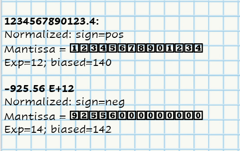
All internal operations will be performed on such normalized values that are stored in internal registers.
Having specified the internal number representation, we can now tackle the four basic algorithms.
Addition/Subtraction
This implementation uses a “nibble-by-nibble” serial algorithm.
Usually, the subtraction is performed by negating the subtrahend and then using the addition. Most known BCD heuristics use 9’s or 10’s complement (subtract each BCD digit from 9 or 10, add one, and then add them). That is also similar to the way processors do subtraction of binary values.
After coding and trying several variations of popular algorithms, I have decided to create a slightly different one, but the one that is more suitable to the architecture that keeps the sign bits separate from their mantissa, and does not store negative numbers as complements. Our implementation of subtraction does not negate the subtrahend. There are many ways to skin a cat, as they say.
Addition and subtraction operations are complementary and are used interchangeably depending on the signs of the addend and augend, or minuend and subtrahend (the former naming a base value, the latter naming a value to be added or subtracted).
First, we align the mantissa so that their digits represent equal decimal weights. The normalized form had them all left-aligned while the exponent specified the position of their decimal points. We must shift the smaller of the two to the right by the difference of their exponents so that we can add ones to ones and tens to tens. However, this could also result in a lesser number being shifted out of existence (ex. 1e20 – 1); we recognize such cases early and return the larger value unchanged.
Since the result may need a new significant digit (as in “9+9=18”), we need to have a nibble pre-allocated for it.
Our code splits up discrete addition and subtraction cases by this heuristic:
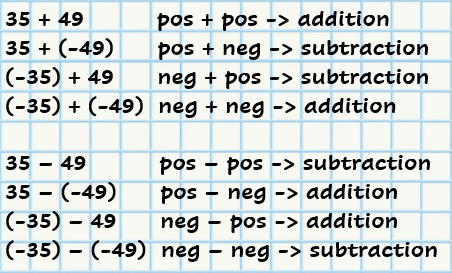
Another twist to subtraction is that we make sure to always subtract a lesser value from a greater one, avoiding the last (MSB digit) “borrow.” When the terms are swapped, the result is the same but negative (like in “10-3=7” but “3-10=-7”)
Although slightly different from the traditional methods of solving the problem, the implemented heuristic is well suited to this architectural implementation, keeping the code readable, simple, and, more importantly, exact.
Multiplication
There are many methods of multiplying two BCD numbers. They range from traditional iterative partial-sum methods to intermediate conversion to binary value and back. There are also different approaches to implementing a multiplier in ASIC and FPGA. However, using an FPGA-embedded multiplier would not be fun, would it?
The multiplication algorithm uses two extra scratch registers: one to store the intermediate product and the other one for a running total of the sums of products. In the outer loop, we multiply a multiplicand with each digit of a multiplier, while in the inner loop, we multiply each pair of individual digits. Each result of these iterations is then summed with the running total.
At this time, we assume that the hardware can multiply a single (4-bit) BCD nibble with another one and return a 2-nibble-wide result. This may be an oversimplification and may change as we start designing the hardware.
The sign of a result is an XOR of the signs of the input terms. The exponent is the sum of the exponents of those terms. Simple.
Division
We use a classic “Shift and Subtract” method to divide two numbers. This method mimics long division. Since the dividend and divisor are already normalized, we do not need to align their decimal digits.
To obtain each quotient digit, we subtract the divisor from the dividend as many times as we can (for as long as the dividend is greater or equal to a divisor) and count. To get the next quotient digit, we shift the dividend to one place (one digit) to the left (thus multiplying it by 10, decimal). Note that many classic “Division by Shift and Subtract” algorithms shift the divisor one bit to the right instead, a process that eventually “eats up” the bottom digits of the divisor, losing the precision.
Once we have found all the quotient digits, the dividend value (now numerically less than the divisor) represents the remainder. If we wanted to, this convenience leaves us with an option to implement a modulus or a remainder function in the future.
Not unlike multiplication, the sign of a result is simply an XOR of the signs of the input terms, while the exponent is a difference of the term’s exponents.
With all four operations, we also need to normalize the result. In the end, the total number of digits might exceed the width of our scratch register, causing a loss of accuracy.
Proof of Methods
To verify our calculations, I have written two projects that you can find in the “Pathfinding/Methods” and “Pathfinding/Proof.”
The code verifies computation against a standard C++ type “double.” This data type is convenient since, when printed, it provides up to 14 or 15 decimal digits of precision. Those are the “control” or “golden” values we compare our results with.
I could have used one of many “Arbitrary Precision Math” packages, but I wanted to take advantage of a C++ built-in type suffices since we don’t need our calculator to exceed its precision. We also don’t need to tie in another potentially large and non-portable package with our sources.
We create a test bench by adding a set of tests to each function we implement. The tests run each function using statically defined values that include several common and many corner case numbers (ex. 0, 1, 0.00000001, 0.99999999).
These values are combined with each other and with varying mantissa and exponent signs.
Additional test sections use purely random values. We use C++11 “std::minstd_rand” to generate the same pseudo-random sequence across different, compliant C++ platforms. That way, our VS and GCC runs will use the same random sequence, and we can compare their outputs as text files.
Although such test coverage is not exhaustive, it seems to be sufficient.
The validator code compares the output of our algorithms with the calculated control value and prints “OK” if the values match exactly, “NEAR” if the values differ by only a magnitude of the last digit (a rounding error), or “FAIL” otherwise.
Since we currently do not perform any rounding, many results are marked as “NEAR,” and this is expected.
It turns out that VS and GCC libraries round numbers differently, so there is a slight mismatch in the control values between those two platforms.
For example, on VS:123456789012345 / 0.1 = 1.2345678901234e+15 vs. +1.2345678901235e+15 NEAR (5e-14)
While on Linux GCC:123456789012345 / 0.1 = 1.2345678901234e+15 vs. +1.2345678901234e+15 OK
(The last number in each line is the control value calculated using a standard VS or GCC library).
I also cross-checked by hand many calculations using SpeedCrunch software, which in this case shows 1.23456789012345e15; and as with many/all other values, the difference is obviously in the rounding digit.
During the development of that code, algorithms, and tests, in the subconscious pursuit of a “perfect match,” I had to keep reminding myself that the goal of this validator was not to match a particular C++ library perfectly but to provide a described and consistent accuracy of the result. At one point, I coded in the rounding function and matched VS control values perfectly. However, the same values would mismatch when compiled with GCC (by the rounding errors), so I decided to keep the code simpler and not do the rounding, for now, implementing only the truncation policy.
There are two major definitions in the validator code: MAX_MANT specifies the number of mantissa digits for input values and the result, and MAX_SCRATCH specifies the number of mantissa digits used in the internal calculation. I call the latter “Arithmetic Scratch Register” since it should likely map to an equivalent register in our final design (at this point, I have not yet defined my CPU).
In the code, you can change those two definitions and see the impact they make on the precision of the results.
Here is the somewhat abbreviated result of the verification: Verification.txt
After getting basic algorithms to work and to match the control values, I could verify successive changes to the code by quickly re-running the tests and spotting functional regressions. Such a verification setup made the development process faster and less error-prone.
Finally, I iteratively rewrote the code, simplifying it into conceptually basic steps (no fancy C++ constructs!) so that we could write a microcode that mimics it. The microcode will be for a simple processor we will design, and the design will be greatly influenced by the kind of operations and data structures (registers) we use in these basic algorithms.
Next article: A Calculator (3): Practical Numerical Methods – Baltazar Studios
Interesting Reads
- HP uses a faster, parallel BCD adder circuitry: http://patft1.uspto.gov/netacgi/nph-Parser?patentnumber=8539015
- An HP division patent: http://patft1.uspto.gov/netacgi/nph-Parser?patentnumber=5638314, where they perform multiple subtractions at the same time to determine the closest divisor that would fit into a dividend or an intermediate remainder.
- BCD Addition and Subtraction is nicely explained here: BCD or Binary Coded Decimal | BCD Conversion Addition Subtraction | Electrical4U, not that we use a different method.
- A really good desktop calculator: SpeedCrunch
- Ken Shirriff peeks into a Sinclair’s 1974 calculator: Reversing Sinclair’s amazing 1974 calculator hack – half the ROM of the HP-35 (righto.com)
- Rounding modes nicely explained: DIY Calculator :: Introducing Different Rounding Algorithms (clivemaxfield.com)