


In the last post, we verified and quantified the precision of the basic four functions (addition, subtraction, multiplication, and division). Now, we can use them as a stepping stone for more complex functions. We can assume they will be available, so our experimentation could simply use built-in C++ functions.
In this article, the third in a series, we will continue with the proof-of-concept, or pathfinding, research.
We will tackle more complex, higher-order functions and investigate methods to compute them. At this point, the focus will be more on the algorithms than on the low-level implementation (that is, we will not be bothered to finesse the code to use a particular hardware register format like BCD; we will simply use a generic “double”).
I have implemented only major functions, not those that could be derived from them. As you will see, there are only a few primary functions that we need. The code also checks for the symmetry of the pairs of functions. The expectation is that running the inverse function on a result should produce the original number, for example, arctan(tan(1.23)) = 1.23.
The theoretical field of numerical methods is wide and mature, and a decent study could take a lifetime (or a Ph.D. thesis), so the algorithms selected for this project do not necessarily represent the best ones available. Most decimal CORDIC algorithms were derived from Jacques Laporte’s web pages. Jacques passed in 2015, but his excellent work on reverse engineering algorithms for HP calculators lives on.
Square Root
Wikipedia: Methods of computing square roots
HP calculators’ algorithm: W. Egbert, 1977 , Volume, Issue May-1977 (hp.com):
- It uses digit-by-digit calculation, never having to go back and correct a digit, hence deterministic time that depends on the number of digits and not on a result’s convergence rate.
- It has additional improvements to speed up the calculation.
- It looks suspiciously like this Japanese method: F. Jarvis, spec4.dvi (shef.ac.uk)
A possibly improved algorithm, but with no accompanied source code: C. Bond, sqroot.pdf (crbond.com)
ZX Spectrum uses Chebyshev polynomials: Logan, O’Hara, The Complete Spectrum ROM Disassembly
- It uses discrete coefficients to approximate sin(x), atan(x), ln(x) and exp(x)
- Based on that, it derives sqrt(x) = (x)^(0.5), where x^y = exp(y * ln(x))
Therefore, a square root could also be implemented using an exponential function.
We will use the Babylonian method: it converges quickly, with most numbers converging in 10-15 iterations. It has two divisions per iteration, but its simplicity makes up for it. The source code is here.
This method starts with an initial guess and squares it. Then it refines that guess depending on the result: if the square of a guess is larger than the original value (“overestimate”), it decrements it, and if it is less (“underestimate”), it increments it. The amount of that correction and the way to calculate it directly affects the quality of the algorithm and the speed of convergence. The process is repeated until we reach the desired accuracy.
The convergence formula that is used is: next_guess = (last_guess + initial_value / last_guess) / 2
We stop when last_guess and next_guess no longer differ.
As an example, here is a table of convergence of sqrt(5.71):
| n | Iteration | last | sx | result | error |
| 5.71 | 0.571 | ||||
| 1 | 0.571 | 10 | 5.2855 | 2.895939371 | |
| 2 | 5.2855 | 1.080314 | 3.182907 | 0.793346404 | |
| 3 | 3.182907 | 1.793958 | 2.488432 | 0.098871646 | |
| 4 | 2.488432 | 2.294617 | 2.391525 | 0.001964209 | |
| 5 | 2.391525 | 2.387598 | 2.389561 | 8.06623E-07 | |
| 6 | 2.389561 | 2.38956 | 2.389561 | 1.35891E-13 | |
| 7 | 2.389561 | 2.389561 | 2.389561 | 0 |
Trigonometric functions
HP35 algorithm: TRIGONOMETRY (citycable.ch) and Cordic (English) (citycable.ch)
ZX Spectrum uses Chebyshev polynomials: The Complete Spectrum ROM Disassembly
- It uses discrete coefficients to approximate sin(x), atan(x), ln(x) and exp(x)
- sin(x) uses 6 constants; exp(x) uses 8; ln(x) and atan(x) use 12 constants
- Based on those, it derives others:
cos(x), tan(x), asin(x), acos(x), **(x) and sqr(x)
cos(x) = sin(PI*W/2), where -1<=W<=1, W is “reduced argument”
tan(x) = sin(x) / cos(x), overflow is cos(x)==0
asin(x): first, tan(Y/2) = sin(Y)/(1 + cos(Y)); then, use atan(Y/2)
acos(x) = PI/2 – asin(x)
Some practical problems with Taylor (or Chebyshev) polynomials are their relatively slow convergence, lots of terms (multiplications and divisions), and thus lots of math for not much precision:
- AC Taylor Polynomials and Taylor Series (activecalculus.org)
- Chebyshev Approximation and How It Can Help You Save Money, Win Friends, and Influence People – Jason Sachs (embeddedrelated.com)
Also, since polynomial solutions only approximate desired functions, their precision wobbles alongside the curve (hence there is a search for a more perfect polynomial that has a good “minimax” property, minimizing the maximal error – a less extreme error wobble across the range); they may be more precise at some points (say, at and around x=0) but are off further you get away from that point.
To reach 12-14 digits of accuracy, we would need to compute many terms (20 or more), which is very computationally intensive.
Here is where the CORDIC algorithm shines. It is not only simple to understand, but with correct optimizations, it is also very fast. In its most optimized form, it uses only basic shifts and adds operations while producing results that are exact to the known precision. CORDIC is not an approximation to a function but a true solution to it.
CORDIC can also be used to compute many other functions, and not only trigonometric.
How CORDIC works?
Suppose we need to find a tangent of 32°. If we graph it, there is a point on the unit circle at P(x,y) for that θ=32°.
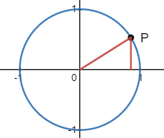
If we somehow find the coordinates of that point P in the cartesian system, we know that the tangent of θ is simply Py/Px. Knowing the tangent, we could also derive sin θ and cos θ using the equivalence formulas.
CORDIC stands for COordinate Rotation DIgital Computer and is based on rotation formulas:
Px = x cos θ – y sin θ
Py = x sin θ + y cos θ
These two formulas tell us how to rotate a point along the unit circle. The first optimization is to simplify those two rotation formulas so that they use only tan θ instead of both sin θ and cos θ:
Px = x – y tan θ
Py = y + x tan θ
For the curious, the exact math of this rewrite can be found here: An Introduction to the CORDIC Algorithm – Technical Articles (allaboutcircuits.com) A take-home point is that the above optimization is almost correct: it will not rotate a point on the unit circle – the point itself will drift out – but the final coordinates will have the same ratio of its x and y parts. It turns out that we care only about that ratio and not the values. The article above mentions a pre-computed scaling factor that could be used to bring the P back onto the unit circle. In that case, computing sin and cos is simpler and more direct.
Let us create a second point, Q, that lies on the x-axis, at (x=1, y=0). We will incrementally rotate it counterclockwise by a certain predefined set of small angles and stop when the total angle of rotation, call it β, reaches the angle we were given as a task to calculate its tangent (θ). The value of tan θ will be the y/x ratio of our rotated point Q. We want β to be as close as possible to θ.
Rotation operations are additive: you can apply many smaller rotations in sequence with the result being the sum of those individual rotations.
A clever trick of CORDIC now comes into play.
We start by making the first rotation of Q by a small angle for which we know the tangent. We could start with 1°, for which tan(1°)=0.01745. Following the rotation formulas, we now need to multiply both Qx and Qy components with 0.01745. Multiplication is an expensive operation that may also contribute to compounding errors when done many times.
Let us look at the problem in this way: we picked 1° since that angle looks nice and round to us. Instead, if we have picked an angle whose tangent was a value that we could multiply with very easily, like 0.1 or 0.01, then we would only need to shift right Qx and Qy. Multiplication with 0.1 in the decimal system (and hence in BCD) amounts to a simple shift by one digit.
That is what CORDIC does: it picks a set of angles for which tangents are 1, 0.1, 0.01, 0.001… Those values correspond to angles of 45, 5.71059, 0.57293… The angles are stored in a table so they can be added to the rotating point Q as its rotation angle approaches the final desired angle.
The result’s precision depends on the number of digits stored in the table and by the algorithmic decision of how close we want to approach the desired angle (the number of iterations).
If we work out our example of 32°, the sequence of computed values would look like this:
| Qx | Qy | New x | New y | Total β | tan θ | θ |
| 1 | 0 | 1 | 0.1 | 5.710593 | 0.1 | 5.710593137 |
| 1 | 0.1 | 0.99 | 0.2 | 11.42119 | 0.1 | |
| 0.99 | 0.2 | 0.97 | 0.299 | 17.13178 | 0.1 | |
| 0.97 | 0.299 | 0.9401 | 0.396 | 22.84237 | 0.1 | |
| 0.9401 | 0.396 | 0.9005 | 0.49001 | 28.55297 | 0.1 | |
| 0.9005 | 0.49001 | 0.8956 | 0.499015 | 29.1259 | 0.01 | 0.572938698 |
| 0.8956 | 0.499015 | 0.89061 | 0.507971 | 29.69884 | 0.01 | |
| 0.89061 | 0.507970999 | 0.88553 | 0.516877 | 30.27178 | 0.01 | |
| 0.88553 | 0.516877097 | 0.880361 | 0.525732 | 30.84472 | 0.01 | |
| 0.880361 | 0.525732397 | 0.875104 | 0.534536 | 31.41766 | 0.01 | |
| 0.875104 | 0.53453601 | 0.869759 | 0.543287 | 31.9906 | 0.01 | |
| 0.001 | 0.05729576 | |||||
| 0.869759 | 0.543287049 | 0.869704 | 0.543374 | 31.99633 | 0.0001 | 0.005729578 |
| 0.869704 | 0.543374025 | – | – | |||
| y/x= | 0.62478023 | |||||
| tan(32°)= | 0.624869352 |
Our result (y/x) compared to the actual tan(32°) differs by only 8×10^-5. Notice that we skipped one table value (for tan θ = 0.001) because the corresponding angle increment of 0.0572, when added to the current running angle β, would have exceeded the target angle of 32°.
Range reduction
Standard trigonometric functions are symmetrical and cyclic, meaning you should get identical results for any positive angles away by a multiple of 360°. Hence, tan(20°) equals tan(380°), but also tan(1.234e10°) equals tan(-80°), which is not as obvious due to the exponential format.
Before starting to compute any trigonometric function, we need to reduce the input angle; we also need to handle large values (with non-zero or large exponents), paying attention to a possible loss of precision that may creep in with that reduction.
Our code implements the heuristic of subtracting 2*PI from the input value until the value is within the (0, 2*PI) range. For larger values (with non-zero exponents), we subtract 2*PI * 10^exp, reducing the exponent as the value gets smaller. Even for large exponents, the convergence to the base range is quite fast.
Function Dependency (trigonometric)
The rest of the trigonometric functions can be derived from this equivalence table. (Source: Wikipedia)
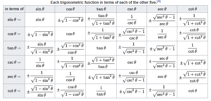
In practice, you do not need to compute both sin θ and cos θ as each one is simply 90° shifted from the other. Having only tan θ suffices to get all other functions.
Inverse trigonometric functions
HP35 algorithm is described here: INVERSE TRIGO (citycable.ch)
These functions can also be computed using Chebyshev polynomials.
If you recall how we calculated tan θ by creating a new point Q at (1,0) and rotating it counterclockwise until it reached the angle θ, inverse trigonometric CORDIC arctan(x) does the opposite: we are given the ratio y/x of a point P located at the unit circle, and we need to find the angle θ that this point makes with the x-axis.
To calculate arctan(x), we create a point P at coordinates (1, x), where x is the input value, and rotate it clockwise until its y coordinate becomes zero (or as close to zero as necessary for the required precision). As we rotate it, we add those small angles. Once y is zero, the total angle of rotation represents arctan(x).
If you look at the code, the algorithm is not immediately obvious due to the shortcuts deployed to simplify BCD arithmetic. The coordinate P has been rotated by a set of angles whose tangents are values easy to multiply with (1, 0.1, 0.01…), and the total rotation is stored in array digits[K], with an index corresponding to that table. The last loop simply sums them up using their positional weights.
Logarithmic and Exponential functions
This is the second major group of functions found on all but the most basic calculators. Just like trigonometry, each function has its inverse counterpart. A convenient property of this group is its rich equivalence table – not unlike the trig functions where we only needed tan θ and its inverse, arctan(x); it turns out that we only need to implement a logarithm and its inverse, the exponential.
For both functions, we again use a variation of a decimal CORDIC.
Logarithm (natural)
As a notation, ln(x) is equivalent to loge(x)
HP35 uses the “Pseudo Division and Pseudo Multiplication” process: LOGARITHM (citycable.ch) which is suitable for BCD architectures.
ZX Spectrum uses Chebyshev polynomials: The Complete Spectrum ROM Disassembly
It uses discrete coefficients to approximate sin(x), atan(x), ln(x) and exp(x)
As with trigonometric functions, ln(x) and eX need to use the same constants and accuracy to assure symmetry.
We are using HP’s method: it is very fast and simple to implement on a BCD architecture. The source code is here.
Although it does not appear so at first sight, the logarithm code is similar to a tangent’s equivalent CORDIC code. Instead of tangent values, its hard-coded lookup tables contain log values.
The basic idea implemented in the log algorithm is that each individual digit of the input value “n” contributes to the result by a certain quantum. An intermediate array digits[M] holds this contribution count (quotients from pseudo-division). The final loop sums up these contributions weighted by this quantum (actual log values stored in a table).
For the more curious, Jacques Laporte explained the algorithm in much more detail: LOGARITHM (citycable.ch)
Logarithm, base-10
log10(x) = ln(x) / ln(10), where ln(10) is a constant 2.30258509299404568402
Alternatively, 10x = e^(x * ln(10))
We will use these formulas to derive the logarithm and exponential of base-10.
Exponential (natural)
Wikipedia: Exponential function
A natural exponential function is defined as y = ex, where e=2.718281828459 (Euler’s number)
This operation can be found written in several different formats: ex, exp(x), or EXP(x), or even e^x.
eX is the inverse of the ln(x), natural logarithmic function, written as loge x, ln(x), or LN(x).
Due to computing imprecision around x=0, many calculators (as well as C++ standard library) implement a function called expm1(x) which is y= ex – 1 instead.
ln(x) and eX need to use the same constants and accuracy to assure symmetry.
HP35 uses the ln(x) algorithm, run in reverse, so to speak: EXP(X) (citycable.ch)
We will follow the HP heuristic and use the same.
Exponential, base-10
Written as yx or y^x, it is often calculated using this formula: yx = e^(x * ln(y))
HP41 is using this formula, and so will we.
Function Dependency (exponential)
Expressing a wide set of functions using a combination the basic ex and ln(x):
| xy | ex | ln(x) | |
| sqrt(x) | x^(0.5) | e^(y * ln(x)) | * |
| 10X | 10^(x) | e^(x * <const>) | |
| log10(x) | ln(x) / <const> | ||
| yX | e^(x * ln(y)) | * |
All hyperbolic functions can also be derived from the same set of basic exponential functions. They operate on the hyperbola rather than the circle (as their trigonometric cousins do), so although they share similar names, they are different kinds of beasts, having more in common to exponential “e” rather than the circular “PI”.
Below is the list of hyperbolic and inverse hyperbolic functions with equations on how to derive them. (Source Wikipedia)
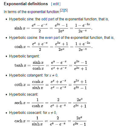
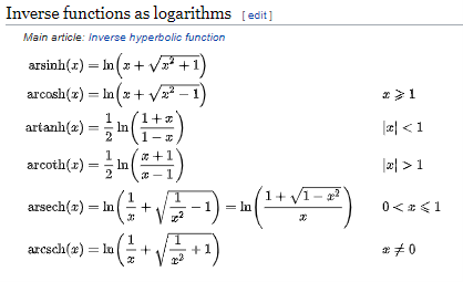
We can get all 18 functions “implemented” for the price of 2 … Isn’t that wonderful?
This should wrap up a brief look at the theory and algorithms of what we are building. It’s time to roll up our sleeves and start with the actual design.
Next article: A Calculator (4): The Framework – Baltazar Studios
Interesting Reads
- An arbitrary precision library: Arbitrary Numerical C++ Packages (hvks.com)
- MATLAB CORDIC library: CORDIC – Approximation of Elementary Functions (fsu.edu)
- Pseudo-division and pseudo-multiplication process (E. Meggitt): Meggitt_62.pdf (citycable.ch)